Statistics with R: install and first steps
Statistical analysis with R
- Review some notions: https://www.khanacademy.org/math/statistics-probability/analyzing-categorical-data
Books
- RStudio : https://rstudio-education.github.io/hopr/starting.html
- R and data sciences: https://r4ds.had.co.nz/
Data
- For this tutorial here
Fancy
- R Markdown to produce beautiful reports: https://shiny.rstudio.com/articles/rmarkdown.html
Download and installation (Ubuntu 20)
Download and install the last release of R from the official website : https://cran.r-project.org/
There is a apt for it:
1
sudo apt install r-base
There also a links for precompiled binary versions, available for Windows, Mac and Linux.
Rstudio
As Rstudio for Ubuntu 20 isn’t available, download the one for Ubuntu18 Jessie.
1
dpkg -i rstudio-1.3.1073-amd64.deb
You might need to run another command to fix dependancies issues.
1
sudo apt --fix-broken install
Launch R interpreter, run Rstudio
Start Rstudio from the launchpad of Ubuntu
or/and
$R runs the R interpreter in your terminal
If you need a graphic interface, dl Rstudio https://rstudio.com/products/rstudio/download/
Run RStudio
First install packages you’ll need to draw plots:
1
    Tools -> Install Packages... ->  and select package you want to install in the dialog box; here "gplots"
Starting key points
- In addition to the visual interface, you can launch instructions directly in the R interpretor (the console) and see the output (crucial for errors)
- Graphs are generated in another window.
- R scripts have the extention .r
you hit a script by running the instruction source()
- You call the help menu by running the instruction help().
Variables
- variables names are Case-senSitiVe
- Missing value is encoded such as NA
- mode() display the variable type numeric or character and lenght() the number of item in the variable
- factor() and levels() are helps to qualify a variable: factor() for what qualitative value of the variable, labels= for labelling the variable
to keep in mind : Variable = (element1, element2, element2, element3,…) it’s like supervariable= [] and a lot of things inthere.
Load data
tips: Cat your file before to see what is the separator used in your data set. For example with a .csv file a “,” or a “;” as separator differs the input syntax: read.csv for “,” and read.csv2 for “;”
1
2
   > smp.c <-read.csv2[file path]
   # smp here is the file in which I lead a set of data with "<-" and the .c method and read from a file.
So with our data: > smp.c <-read.csv2(“data/smp1.csv”)
To check the data integrity :
1
    > str(smp.c)  ~~~R  'data.frame':	799 obs. of  9 variables:  $ age      : int  31 49 50 47 23 34 24 52 42 45 ...  $ prof     : Factor w/ 8 levels "agriculteur",..: 3 NA 7 6 8 6 3 2 6 6 ...  $ dep.cons : int  0 0 0 0 1 0 1 0 1 0 ...  $ scz.cons : int  0 0 0 0 0 0 0 0 0 0 ...  $ grav.cons: int  1 2 2 1 2 1 5 1 5 5 ...  $ n.enfant : int  2 7 2 0 1 3 5 2 1 2 ...  $ rs       : int  2 2 2 2 2 1 3 2 3 2 ...  $ ed       : int  1 2 3 2 2 2 3 2 3 2 ...  $ dr       : int  1 1 2 2 2 1 2 2 1 2 ...  ~~~
Visualizations
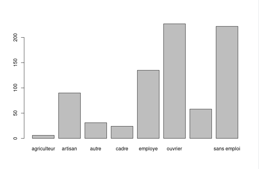
barplot
1
    > barplot(table(smp.c$prof))
The same thing as table in the console:
1
    > table(smp.c$prof)
1
2
3
4
      agriculteur            artisan              autre              cadre            employe            ouvrier prof.intermediaire
                 6                 90                 31                 24                135                227                 58
       sans emploi
               222
vocabulary:
http://vita.had.co.nz/papers/layered-grammar.pdf
